Unsupervised Kernel Regression (UKR)

In general, the domain of manifold learning addresses the problem of finding a lower dimensional (latent) representation of a set of observed data and the corresponding functional relationship .

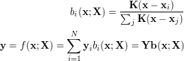
Unsupervised Kernel Regression (UKR) is a recent approach to learning non-linear continuous manifold representations. It has been introduced as an unsupervised formulation of the Nadaraya-Watson kernel regression estimator by Meinecke, Klanke et al. and further developed by Klanke. It uses the Nadaraya-Watson estimator as mapping between latent and observed space:

(1)

This estimator realises a smooth, continuous generalisation of the functional relationship between two random variables and described by given data samples . Here, is a density kernel like Gaussian or Quartic and contains the corresponding bandwidths. Whereas the choice of the kernel is of relatively low importance, the bandwidth plays a more crucial role in the original estimator.

UKR now treats (1) as a mapping from the latent space of the represented manifold to the original data space in which the manifold is embedded and from which the observed data samples 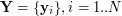are taken. The associated set 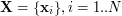now plays the role of the input data to the regression function (1). Here, they are treated as \textit{latent parameters} corresponding to . As the scaling and positioning of the 's are free, the formerly crucial bandwidth parameter becomes irrelevant and we can use unit bandwidths.

The UKR regression function thus can be denoted as

(2)

where is a vector of basis functions representing the effects of the kernels parametrised by the latent parameters.

The training of the UKR manifold, or the adaptation of respectively, then can be realised by gradient-based minimisation of the reconstruction error

(3)

where .

To avoid the trivial minimisation solution by moving the infinitely apart, several regularisation methods exist. Here, the most outstanding to mention is UKR's ability of very efficiently performing a leave-one-out cross-validation, that is, reconstructing each without using itself. To this end, in the calculation of (cf. (3)), the only additional step is to zero its diagonal before normalising the column sums to 1.

n=0	n=5	n=10	n=20	n=100
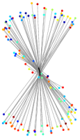
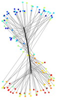
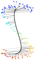
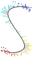
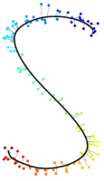
Fig.1: Progress of UKR training of a "noisy S" after n=0,5,10,20,100 gradient steps. Depicted are the reproduction of the one-dimensional UKR latent space (black line) and the corrsponding training data points (points, colours visualise the value of the 1D-latent parameter).

Note that, for a preselected density kernel, the reconstruction error (3) only depends on the set of latent parameters . Thus, minimising w.r.t. optimises both the positioning of the latent parameters 's and the shape of the manifold at the same time. In this feature, UKR differs from many other manifold representations which usually require alternating projection and adaptation steps.

As gradient descent often suffers from getting stuck in poor local minima, an appropriate initialisation is important. Here -- depending on the problem -- i.e. PCA , Isomap or Local Linear Embedding (LLE) are usually good choices. These methods themselves are quite powerful in uncovering low-dimensional structures in data sets. In contrast to UKR indeed, PCA is restricted to linear structures and Isomap as well as LLE do not provide smooth mappings into the data space.

An inverse mapping from data space to latent space is not directly supported in UKR. Instead, one may use an orthogonal projection to define a mapping which approximates .

UKR is presented in more detail in: MeinickeKlankeMemisevicRitter2005-PSF, KlankeRitter2006-ALK, KlankeRitter2007-VUK, Klanke2007-LMW.